Choosing Temperature Transmitters: Sensor Inputs, Accuracy and Outputs
Author
Date Published
Reading Time
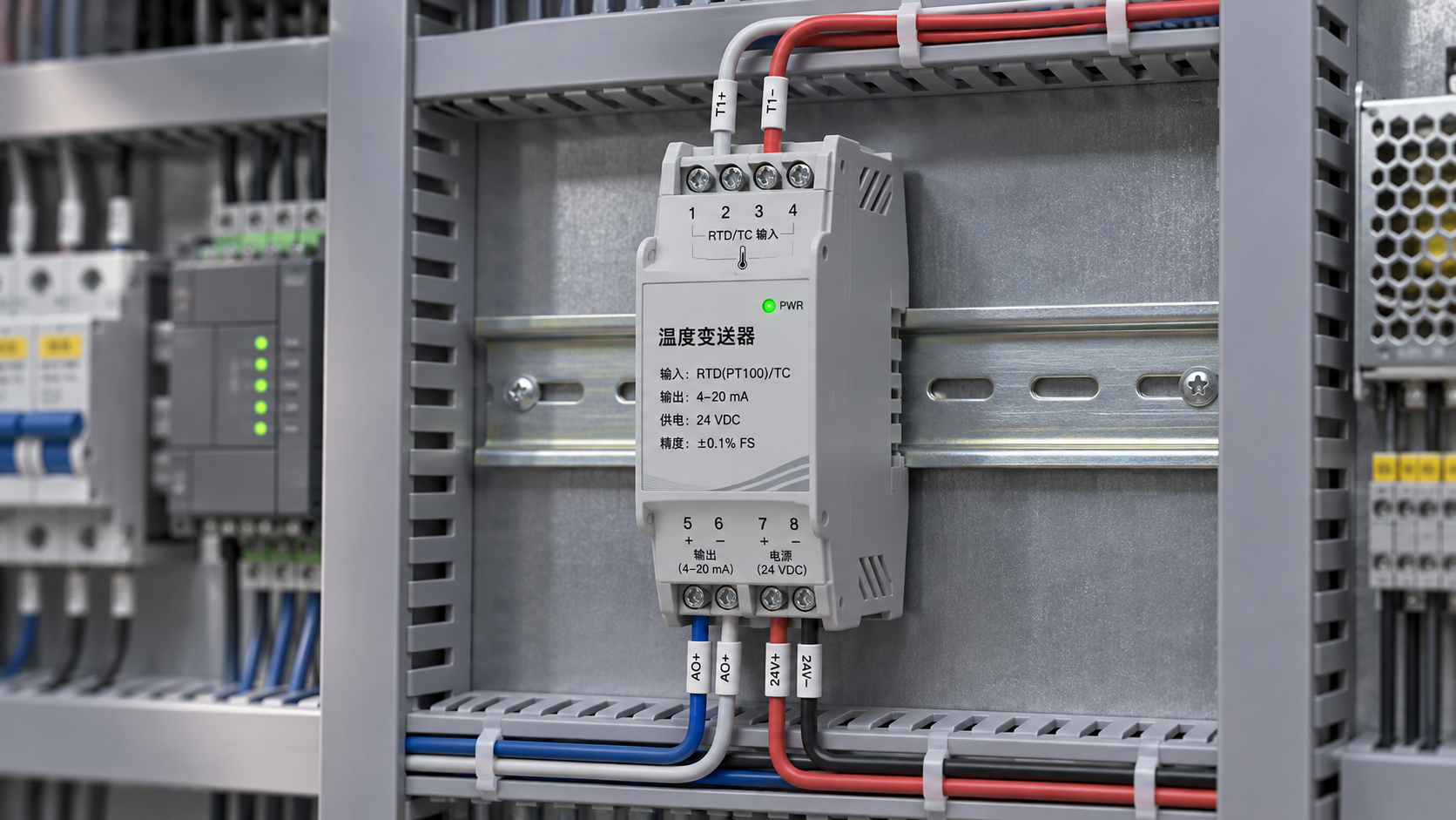
Select temperature transmitters by matching the complete measurement chain: sensor type and wiring, required accuracy over the operating range, output compatibility, and the conditions at the installation point. A transmitter with an impressive reference accuracy can still produce a poor measurement if its input configuration, ambient rating, sensor connection, or output load is unsuitable.
Start with the temperature range that matters to the process, then establish the allowable error at the control system input. Compare transmitter specifications at those actual conditions, including sensor tolerances and ambient temperature effects. Finally, confirm that the selected output, power supply, mounting arrangement, and diagnostic behavior fit the existing system.
Match the input to the sensor and its wiring
An RTD measures temperature through a change in electrical resistance. A thermocouple generates a small voltage related to the temperature difference between its measuring junction and the reference junction. The transmitter must support the exact sensor type and its expected range; a universal input is useful only when the required sensor curve and wiring arrangement are included in its configuration options.
For an RTD, a two-wire connection includes lead resistance in the measurement. That error grows with cable resistance and is particularly relevant when the sensor is far from the transmitter. A three-wire circuit compensates for lead resistance by assuming the relevant leads have closely matched resistance; mismatched wires or corroded connections undermine that compensation. A four-wire measurement separates the current and voltage paths and largely removes lead resistance from the reading, provided the transmitter supports the connection.
Thermocouple selection requires the correct type throughout the measurement chain. Extension or compensating cable must be suitable for that thermocouple and installed with the correct polarity. Joining dissimilar conductors creates additional junctions, so terminal temperatures and wiring transitions affect the result. The transmitter’s cold-junction compensation must reflect the temperature at the actual transition to its input terminals. A device mounted near a hot surface or exposed to uneven airflow can develop terminal gradients that weaken compensation.
Also establish the desired response to a broken or shorted sensor. A detected open circuit can drive the output to a configured fault level, but short-circuit detection is sensor- and transmitter-dependent. A shorted thermocouple circuit can produce a plausible voltage, so an open-sensor diagnostic alone does not guarantee detection of every sensor fault.
Read accuracy against the actual measurement range
Accuracy figures are only comparable when their reference conditions and units are understood. A specification may be expressed in degrees, as a percentage of the configured span, or as a percentage of the reading. It may apply to a particular sensor type and input range, with separate allowances for analog output conversion, ambient temperature, and long-term drift.
For example, an error stated as a percentage of span represents a larger temperature error when the configured span is wider. An error stated in degrees remains the same numerical amount across different spans. Use the manufacturer’s applicable specification for each input type and configured range; do not assume the most favorable number in a general product summary applies to every sensor.
The transmitter is only one contributor to measurement uncertainty. The sensor’s tolerance, calibration condition, lead resistance, cold-junction compensation, and installation all affect the final result. The receiving analog input has its own error as well. When a defensible uncertainty estimate is required, combine the relevant contributions using a method appropriate to their stated limits and statistical properties. Simply adding every figure gives a conservative bound only when the figures are compatible limits; a root-sum-square calculation requires justified assumptions about independence and distributions.
As an illustration, a transmitter configured for 0–200 °C with an input error limit of ±0.1% of span contributes up to ±0.2 °C from that stated term alone. If an analog output error is specified separately, include it as directed by the data sheet. The sensor and installation errors remain additional contributors. This arithmetic describes the stated example, not a typical device specification.
Reference conditions are not field conditions
A transmitter mounted in a warm enclosure can perform differently from its stated reference accuracy. Review the ambient operating range and the temperature coefficient over the expected enclosure temperature, not just the process temperature. Self-heating, sunlight, nearby equipment, and restricted ventilation can make enclosure air and terminal temperatures higher than surrounding air.
Resolution is also distinct from accuracy. A display or digital output that changes in small increments does not prove that the measured value is close to the true temperature. Likewise, repeatability describes consistency under stated conditions; a repeatable reading can still carry a calibration offset.
Choose the output for the control system
A 4–20 mA current loop is a common choice for transmitting a scaled value over industrial wiring. Confirm whether the transmitter is loop powered or separately powered, the available supply voltage, and the resistance of the complete loop. The supply must leave enough voltage across the transmitter after accounting for the voltage drop through the receiving input, barriers, wiring, and any other series devices.
For a linear temperature output, 4 mA represents the lower range value and 20 mA the upper range value. A narrower configured span gives a larger current change for a given temperature change, which improves the use of the receiving system’s input resolution. It also brings the limits closer to the process: temperatures outside the configured range require an agreed behavior for overrange, underrange, and fault conditions. Confirm both the transmitter’s limits and the receiving system’s interpretation of those signals.
HART communication can add configuration and diagnostic information to a compatible analog loop while retaining the current signal for the primary measurement. The host, interface, and loop impedance must support the communication arrangement. A digital fieldbus or network output can carry additional measurements and status information, but it requires a compatible host, network design, power arrangement, and device integration files where applicable. Choose the information that needs to reach the control system before specifying the communications protocol.
Voltage outputs require a compatible input range and adequate attention to voltage drop and electrical interference. They may suit short connections inside an enclosure; over longer runs, cable resistance, grounding, and input impedance deserve closer review. For any output, confirm whether isolation is provided between sensor input, output, and power. Isolation can reduce unwanted current paths, but its rating and purpose must match the installation.
Mounting position changes the trade-off
A head-mounted transmitter shortens the low-level sensor wiring and places the output conversion near the measurement point. That arrangement is attractive for thermocouples and long cable runs, provided the connection head stays within the transmitter’s ambient limits. Heat conducted along a probe or trapped in a sunlit head can make the local temperature substantially different from the surrounding air.
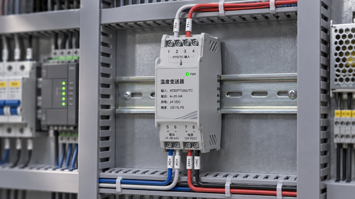
A DIN-rail transmitter in a protected cabinet is easier to access for configuration and replacement, and the cabinet may offer a more stable environment. The sensor leads must then reach the cabinet. RTD lead resistance, thermocouple extension cable, electromagnetic interference, and cable routing become more significant as that distance increases. Neither location is automatically superior: compare the conditions at both ends of the proposed cable run.
Mechanical fit deserves the same attention as electrical compatibility. Confirm mounting dimensions, terminal access, enclosure ingress protection at the installed assembly, and available cable entries. Vibration and moisture at the mounting point can damage connections even when the transmitter itself has a suitable ambient temperature rating. For hazardous locations, select equipment and installation methods whose approvals and conditions of use match the classified area; the transmitter, enclosure, barriers, and wiring form part of that assessment.
Separate sensor response from transmitter response
A fast transmitter cannot compensate for a slow sensor assembly. Thermowell wall thickness, insertion depth, sensor contact, and the surrounding medium all influence how quickly the sensing element reaches process temperature. A probe exposed to the temperature of a pipe wall, for example, does not necessarily represent the fluid temperature without a suitable installation.
Digital filtering can steady a noisy output, but it also delays the reported response to a real temperature change. Compare the transmitter’s update rate and configurable damping with the needs of the control loop or alarm function. Excessive damping can hide short excursions; too little can produce unstable control or nuisance alarms. Establish the intended setting during commissioning rather than comparing response specifications in isolation.
Verify configuration and fault behavior before release
Record the sensor type, wiring mode, measurement units, lower and upper range values, output direction, filtering, and fault action as part of the instrument configuration. A transmitter configured for the wrong RTD curve or thermocouple type can display a credible value while introducing a systematic error. Where a custom sensor calibration is used, confirm that the device accepts the required coefficients and that the receiving system uses the same units and scale.
A practical acceptance test injects known resistance or millivolt signals at several points across the configured range and compares the output with the expected values. For thermocouple simulation, account for reference-junction compensation in both the simulator and transmitter; otherwise the test setup itself can introduce an offset. Exercise the configured open-sensor fault and verify that the control system identifies it correctly. An end-to-end test with the installed sensor provides additional evidence about wiring and integration, while a calibrated input simulation isolates the transmitter’s performance.
Before substituting one model for another, compare the configured input and output, supply and load limits, physical fit, isolation, diagnostic behavior, and ambient effects. Two transmitters with the same nominal 4–20 mA output can behave differently when a sensor fails or the measured temperature moves outside the configured range.
Expert Insights

Chief Security Architect
Dr. Thorne specializes in the intersection of structural engineering and digital resilience. He has advised three G7 governments on industrial infrastructure security.
Related Analysis
- Nov 22, 2026McKinsey: India Needs Up to $400 Billion to Meet Steel Capacity Growth GoalAuthor :
- Nov 22, 2026Choosing Geotextile Fabric for Landfill Drainage and Liner ProtectionAuthor :Environmental Engineering Director
- Nov 21, 2026Japan's Steel Exports Could Fall to Lowest Level Since 1999 in 2026Author :
Core Sector // 01
Security & Safety
- Choosing Ambient Air Monitoring Equipment: Pollutants, Range and AccuracyAuthor :Precision Metrology Expert

- Surface Roughness Tester Price: What Drives the Cost of a Purchase?Author :Precision Metrology Expert

- Choosing Temperature Transmitters: Sensor Inputs, Accuracy and OutputsAuthor :Precision Metrology Expert

- FCC Votes to Bar All China-Based Labs From Testing Electronics for US MarketAuthor :Precision Metrology Expert

- Choosing Contact Temperature Instruments: Accuracy, Range, and Response TimeAuthor :Precision Metrology Expert

- How to Validate Third-Party Flow Meter Vibration Data for Humid ClimatesAuthor :Precision Metrology Expert

- Are IEC Standards and ATEX Mandatory for Overseas Pressure Instruments?Author :Precision Metrology Expert

- How to Verify ATEX Pressure Transmitters for Overseas Oil and Gas SitesAuthor :Precision Metrology Expert